Progress on the Image Polyline Conversion has been moving forward. We ultimately developed 2 methods of processing, and a third is nearly finished. Here are the current working titles:
- RGB Grid Matrix Method
- Randomized Node Method
- Averaged Linear RGB Method
1.) The RGB Grid Matrix Method has already been documented last week, and currently we are calibrating using an image of Samuel Clemens. It has several spots where the code needs to navigate narrow isthmuses and islands of RGB content, so it is an ideal test project.
To reiterate the previous post, the Matrix Grid system uses pre-extracted RGB grid from the driver image, then calculates the nearest neighbors’ maximum values until the grid is consumed. This process is pseudo-recursive, and reads a sub-grid at each local check.
2.) The Randomized Node Method is a new method developed because the Grid Matrix system lacked a smooth way to transition between long gradients. This new technique sacrifices the elegance of the UV grid to distribute a preset number of nodes randomized throughout the image on an inverse squared RGB contrast value. Then that new point becomes the start for the same test process until the whole image is utilized.
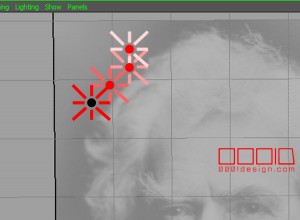
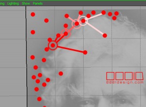
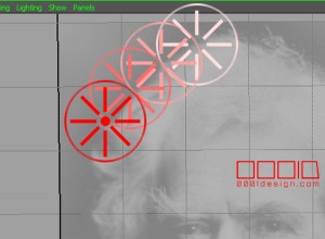
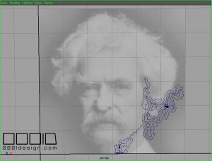
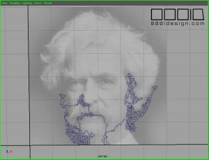
3.) The latest in-progress method averages the RGB values along a straight line segment on the image. This Averaged Linear RGB Method recursively propagates by testing a 360 degree spread of straight lines and the RGB values along those lines. This method is unique, because unlike the previous two, this can tell if a path has a valley of lighter colors. Only the strongest dark areas will be selected before continuing on. Eventually all regions are filled with lines as it checks against a global array of coordinates.
All three methods have pros and cons. All three have slight aesthetic differences. Method 1 leaves large white spots and delicately plays with Gestalt. Method 2 has beautiful gradients but leaves large line segments to fill in the vestigial spots. Method 3 is still in progress, but early tests show a proclivity for fragile fingerprint-style nested curves and contours.
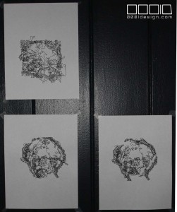
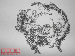
Utilizing the “Monster” CNC machine, three drawings have already been produced. These three images document only the first and second methods, for the third method still has not been finished. In the image below, the bottom two drawings are Method 1, and the top image is a mis-calibrated Method 2.
Unfortunately, we are still calibrating the Monster CNC device, so some of the lines are off. This is more evident in the top drawing, but all have flaws. Hopefully in the following days, these problems will be resolved.
Lastly, since we do not have any CNC drawings of the third method, here are few in-progress screenshots.
Much progress has been completed since these screenshots were taken. Hopefully by tomorrow, a rough draft version of the code will be executable. The major advancement is the ability for the “fingerprinting” to have variable thicknesses and offsets.
Also, the design of the third method was a challenge, because one of the givens is to reject any imposed programmatic randomness. The process is completely repeatable, whereas the first two methods always result in a slightly different pattern. We can see advantages to randomness for this exercise, but just for shits and giggles, this third technique was to avoid it.

![[0001D] Maya MEL Single Polyline Path Image Optimizations](https://www.nickpisca.com/sherpa/wp-content/uploads/2015/03/IMG_9982sfw.jpg)

Trackbacks/Pingbacks